Time Series - Logistics
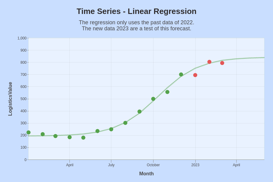
The task here is to assess a regression model using with test data. Particularly for the use case when at the beginning of a month the data of the previous month are available.
The problem addressed here is to compute the model only with the model data. Further, the chart should clearly show which data belong to the model and which belong to the test.

A Linear Regression was added to the 'model' data of the time series leading to a forecast. Afterwards, the chart was updated with test data.
Solution idea and some details
Create file with aggregated, monthly data
The solution here is essentially an extension of the previous example on Time Series Update.
Logistic Function For Time series
In fact, there is nothing special here about time series, but a mapping from the time series to integers and then back to the time series. The point is to make these two mappings most efficiently and readable in the coding.
The Logistic function used here was coded as
y = M * (1 / (1 + np.exp(-s * X)))
with
M = MaximumMarketSize
s = Steepness (of the slope)
Optimization
There are several optimization libraries available in Python which can be used for fitting a curve and particularly for fitting the Logistic function. Here, the library scipy is used.
from scipy.optimize import curve_fit
The optimization can be optimized with both an initial set of parameters (p0) and boundaries for these parameters (bounds)-
popt, pcov = curve_fit(LogisticsFunction, dfTL.X, dfTL.Y, p0=p0, bounds=bounds)
The parameters optimized (popt) are returned from the optimizer together with the parameter covariance (pcov).
Handling the Time Series
Shortly, before handing over to the optimizer, the fore each row of the time series an integers is created.
dfTL["X"] = np.arange(0, dfTL.shape[0], 1)
This slightly enhanced dataframe is handed over to the optimizer.
As the date remains within this dataframe, that’s all that needs to be done. The original time series remains in the data frame and is used for the X-Axis in the subsequent chart.